Untangling graphical pangenomics
For five years I have worked on a simple, universal, graphical model for pangenomic reference systems: the variation graph. I haven’t been alone. This work began as part of the GA4GH data working group (GA4GH-DWG), which spent several years debating and proposing various graphical pangenomic models. After I built a working system based on the variation graph model, vg, many members of that groups then joined me to continue its development, forming the vgteam. Although the data formats produced by our effort was never ratified as a standard by the GA4GH, they are now in wide use.
This group continues to build and refine reference implementations of bioinformatic methods based on the variation graph model. Together, we have demonstrated that these approaches can significantly improve read mapping to variant alleles, and although this benefit is subtle when the reference graph is built from small variants detected by alignment against a linear reference, it becomes substantial when the graph is built from whole genome assemblies representing all types and scales of variation. These methods and the lessons learned developing them are thus of critical importance to the construction of unified data models for de novo assemblies of large genomes that are rapidly being generated using third generation sequencing technologies.
A model for graph genomes
A variation graph combines three types of elements in a pangenomic data structure. We have DNA sequences (nodes), allowed linkages between them (edges), and genomes (paths) that are walks through the graph. Nodes have identifiers, which are numeric, and paths have names, which are text strings. One concession is made to reflect the genomic use of these graphs. They are bidirectional, and represent both strands of DNA, so positions refer to either the forward or reverse complement orientation of nodes. This means that there are four kinds of edges (+/+, +/-, -/-, -/+), each of which implies its own reverse complement.
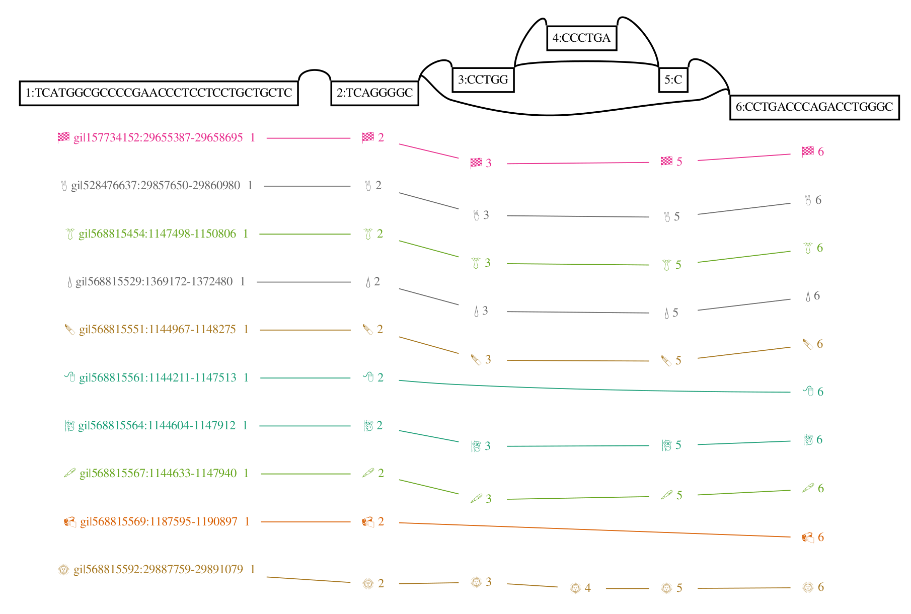
There are many ways to visualize these graphs, but perhaps the most instructive here is the first one that I developed, based on graphviz’s dot. This rendering (from my thesis, Graphical pangenomics) shows a fragment of a variation graph built from a progressive alignment of the GRCh38 ALT haplotypes for HLA gene H-3136. We don’t have any inverting edges or cycles, but we do see a feature that’s impossible to express in VCF: nested variation. Above, we see the core of the graphical structure. Below, paths are represented by the sequence of node identifiers they pass through.
Schema based data formats for variation graphs
Along with Adam Novak (who helped to make it bidirectional), I first implemented this model in a short protobuf schema. By compiling this schema into a set of class libraries, we built both an API and a set of data types for graph-based genomics directly from the schema. This approach was very much in line with the activities of the GA4GH-DWG community discussions (for instance: 1 2), which aimed to build schema-based interchange formats rather than basic textual ones.
The schema includes both the basic graph implementation (the .vg format, which is equivalent to a subset of GFAv1), and Alignment object definition that allows us to use these graphs in resequencing. Others have extended this schema to support particular applications such as genotyping and graph structure decomposition. Many more have used it in their own projects. Of particular note are two graph based read aligners, GraphAligner and PaSGAL, which implement efficient heuristic and exact long read alignment against sequence graphs. These methods, as well as vg, emit the GAM (graphical alignment/map) format. GAM extends the concept of a pairwise sequence alignment record to the case of sequence alignments to the graph. As with all data formats in vg, GAM has both textual (in JSON) and binary (protobuf) versions. Mirroring the .vg equivalence with GFA, GAM is semantically equivalent to the nascent line-based GAF format that has recently been proposed. The vg schema and an independent API for reading and writing files in it now lives in libvgio.
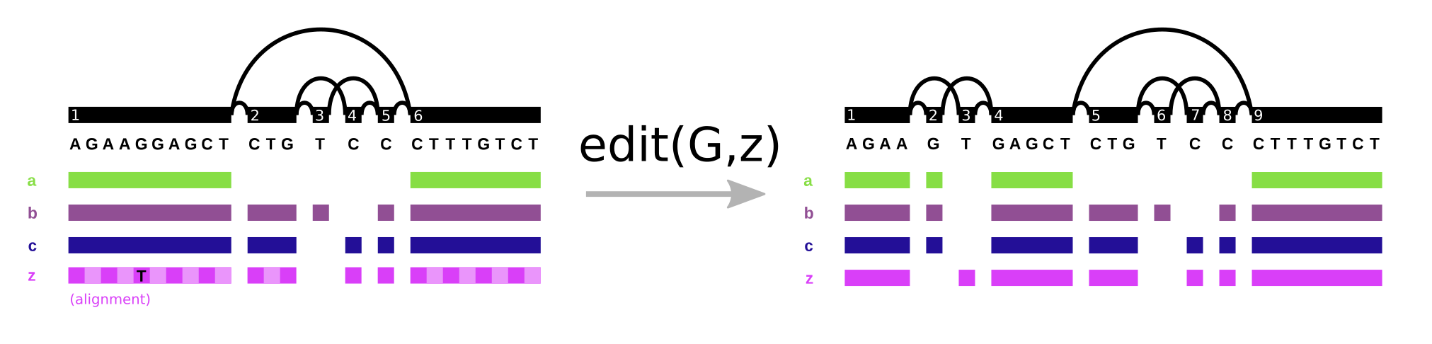
In vg, the Path data type plays double duty. It represents both walks through the graph and the base level alignment of a sequence to the variation graph (it’s one of the components of the Alignment object). We see the same pattern in GFA/GAF. Path steps in GFA have cigar strings, as can alignment records in GAF. However, it’s important to note what this allows us to do. We can support the “fundamental” operation of variation graphs, edit. Here, we augment the graph on the left (G) with alignment z, that includes a SNP allele, yielding the graph on the right:
With this operation and an aligner, we can progressively build variation graphs (as in vg msga).
If we build a variant caller that emits genotypes as sets of Paths, then we can directly use the output of the variant caller to extend the reference system with the same function (as in vg call).
Pangenomic model choice
The variation graph model is designed to be as simple as possible. It makes no assertions about graph structure or coordinates. This design was intentional, because simplicity allows for generality. It is possible to use virtually any kind of sequence graph as the basis for a variation graph. In vg, we have implemented constructors for variation graphs that start from VCF files and references, de Bruijn graphs, string graphs, multiple sequence alignments, RNA splicing graphs, and whole genome alignments. If you can build a sequence graph, vg can use it as a reference system.
Although graphs built from linear references and VCF files were our primary focus, in our paper on read alignment to variation graphs, we demonstrate that we can use vg to align long PacBio reads from a held out strain to a whole genome alignment graph (made by Cactus) built from six other de novo S. cerevisiae assemblies. My thesis covers many other examples, including a freshwater viral metagenome, a bacterial pangenome, a structural variation graph, a yeast splicing graph, and a human gut microbiome.
This generality came at a cost of increased development time, as there was more for us to learn and discover. However, as the collaboration driving vg progressed, we learned how to handle this complexity. We found that, while the variation graph is an ideal data integration system, we may need to construct technical transformations of genome graphs to enable efficient read alignment against them. In general, these graphs are strict subsets of larger graphs, with reduced complexity. But they may also involve the unfolding or duplication of complex regions, so as to reduce the path explosion that can occur when many variants occur in proximity. We preserve a mapping between the technical and base graphs, using each in its optimal application. It would trivialize our work to suggest that this is always easy. Our success indicates that it is possible and more expedient than was expected by groups that chose to restrict their pangenomic model a priori.
Paths provide coordinates and memory to genome graphs
Many genomics researchers, when confronted with genome graphs, immediately worry that there will no longer be any stable coordinates to place annotations on the graph or relate it to known genomes. Graphs are just representations of multiple sequence alignments. Alignments are capricious and can change depending on scoring parameters, order, or the structure of input sequences and their overlaps. We should not trust that the same input sequences will result in the same graph.
In the GA4GH-DWG, we spent most of a year (2014-2015) debating different data models for reference pangenomes that attempted to resolve this issue. Many participants proposed models that preserved a preexisting reference coordinate system directly in the structure of the graph. However, few provided working implementations to back up their argument, and so these conversations mostly addressed hypothetical issues.
In response, I proposed the first prototype of vg itself and demonstrated that I was able to use it to align reads to a graphical genome model built from the whole 1000 Genomes Project phase 3 release. Because of its generality, the variation graph model could consume any of the other data models that had been proposed, which made it of immediate practical use to drive the comparative evaluations between different graph models that were the primary research output of the GA4GH-DWG.
Variation graphs address the pangenome coordinate problem in the most simple way possible. As long as they embed reference paths that cover most of their space, such that no graph position is “far” from a reference position, we can derive reference relative coordinates for positions on the graph. If we build the graph a different way from the same sequences, the relationship between coordinates in different reference paths changes, but we do not gain or lose any coordinates. This solution is inelegant (we don’t get a single, immutable coordinate hierarchy), but practical and extremely flexible.
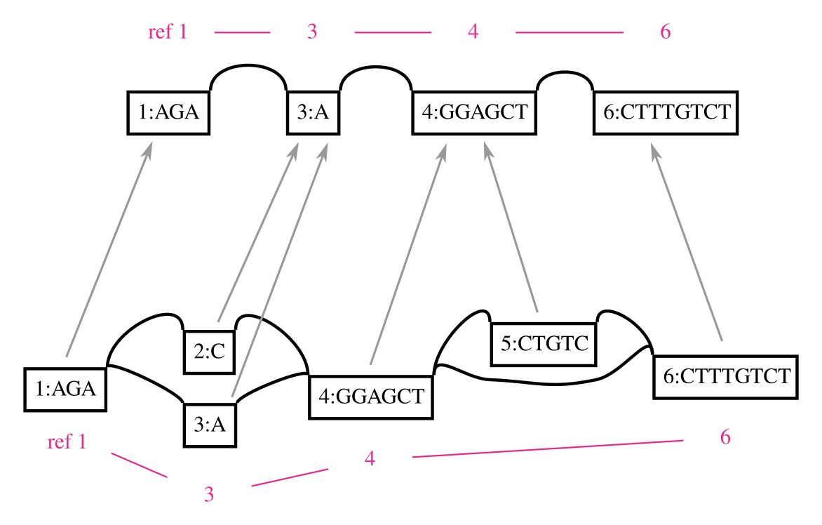
A genome graph is just an alignment of linear sequences, and these remain linear even if they are embedded in a graph. We can use this property to project results obtain relative to genome graphs to linear sequences, such as by “surjecting” alignments from the graph into a subset of reference paths that overlap most of the graph (from GAM to BAM). Many analyses in my thesis used this feature, and it is a key aspect of our ongoing work on ancient DNA. In this context, the graph is simply a black box that is used to reduce reference bias during alignment. To illustrate this concept, the following figure shows a surjection function in terms of node space for a graph and the subgraph corresponding to its embedded path. This kind of projection will work for any pair of graphs with the same embedded path.
This feature also addresses another key shortcoming of genome graphs. Graphs built from sequences and linkages between them are memoryless, and allow recombinations of alleles that are very unlikely to exist in reality. The paths in the variation graph address exactly this issue, and provide long range structure to the object that would be lost if it were simply a graphical model.
Although paths are expensive to store, in a given species most haplotypes at a given locus will be similar, and we can exploit this to compress genomes into haplotype indexes like the GBWT that use only a fraction of a bit per basepair of stored sequence while providing linear-time haplotype matching and extraction functionality. This result suggests that it might be tenable and even desirable to store all the sequences that we used to build a pangenome, even if these number in the many millions.
The next phase of graphical pangenomics
Now, five years into my experience in this subfield, we are at an inflection point. Far from being a curious way to reduce reference bias against small variants, vg and other graphical genomic methods are poised to become a key toolset for managing and understanding an oncoming deluge of whole, large, genomes from vertebrates, including humans. To address this need, I have spent much of the last year working on a series of tools that allow us to construct and manipulate variation graphs representing whole genome alignments of large numbers of large genomes.
The first, seqwish, consumes alignments made by minimap2 over a set of sequences and produces a variation graph (in GFA format) that losslessly encodes all the sequences (as paths) and their base pair exact alignments (in the graph topology itself). This method is several orders of magnitude faster than equivalent methods like Cactus, and is more flexible than de Bruijn graph based methods like SibeliaZ. Although it is very much still a prototype, I am now reliably able to apply seqwish to collections of eukaryotic genomes such as human, medaka, and cichlids. For testing, I construct pangenomes for yeast on my laptop in a few minutes, a task that used to take up to a day on a large compute node. Still, its performance can be improved greatly, and the complete range-based compression of its data structures (using Heng Li’s awesome implicit interval tree) will allow it to scale to the construction of a lossless pangenome from hundreds of human genomes. Because it exactly respects its input alignments, seqwish can act as a self-contained kernel in a pangenomic construction pipeline. Once it is sufficiently optimized, the difficulty will lie in structuring and selecting the best set of alignments for a given pangenome.
A key failing of vg has been its in-memory graph model, which can consume up to 100 bytes of memory per input base of the graph. Although acceptable for a starting PhD project and proof of principle methods, this is not scalable to the problems that we routinely apply vg to. We have had to work around this in various ways, such as by subsetting graphs to single (human scale) chromosomes, by using larger memory machines, or by transforming the graph into static succinct indexes like xg. Last winter, at the NBDC/DBCLS BioHackathon in Matsue, Jordan Eizenga and I decided to tackle this issue by building a set of dynamic succinct variation graph models. These present a consistent HandleGraph C++ interface, and can be used interchangeably with any algorithms written to work on this interface, of which there are now many. The result of my own work on this topic is odgi, which provides efficient postprocessing for the large graphs built with seqwish. Currently, this method supports the difficult steps of graph topological sorting, pruning, simplification, and kmer indexing. I plan to extend it to support read alignment and progressive graph construction, to complement seqwish and other emerging methods like minigraph.
To illustrate these two tools, consider the set of genomes from the Yeast Population Reference Panel. Here, taking only the cerevisiae genomes, we run minimap2, filter the alignments to remove short alignments <10kb, then induce the variation graph with seqwish and render an image of the output with Bandage:
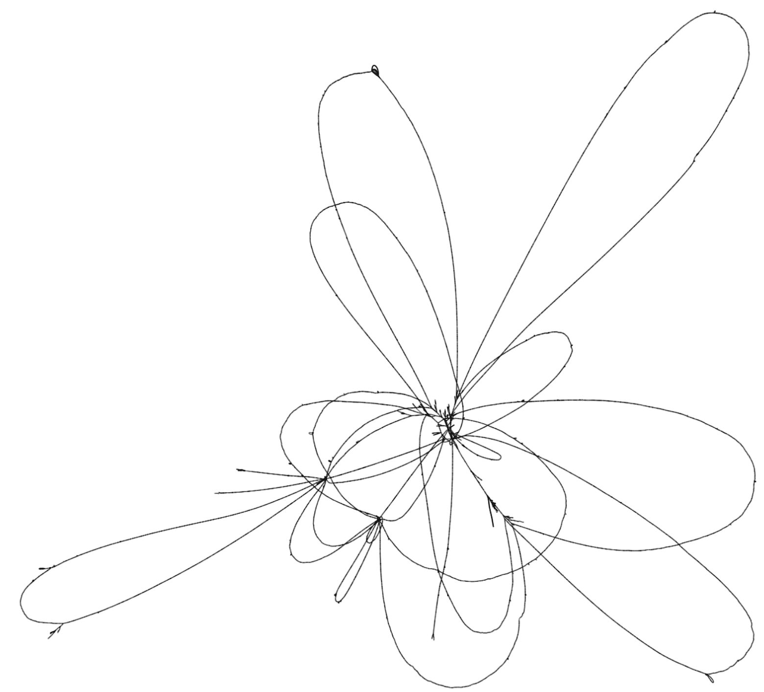
This shows a relatively open graph, with some collapse and some apparently unaligned chromosome ends (perhaps because of our length filter).
Rendering with Bandage can take an extremely long time and the resulting graphs are difficult to interpret because it is not easy to view the relationship between different embedded paths in the graph.
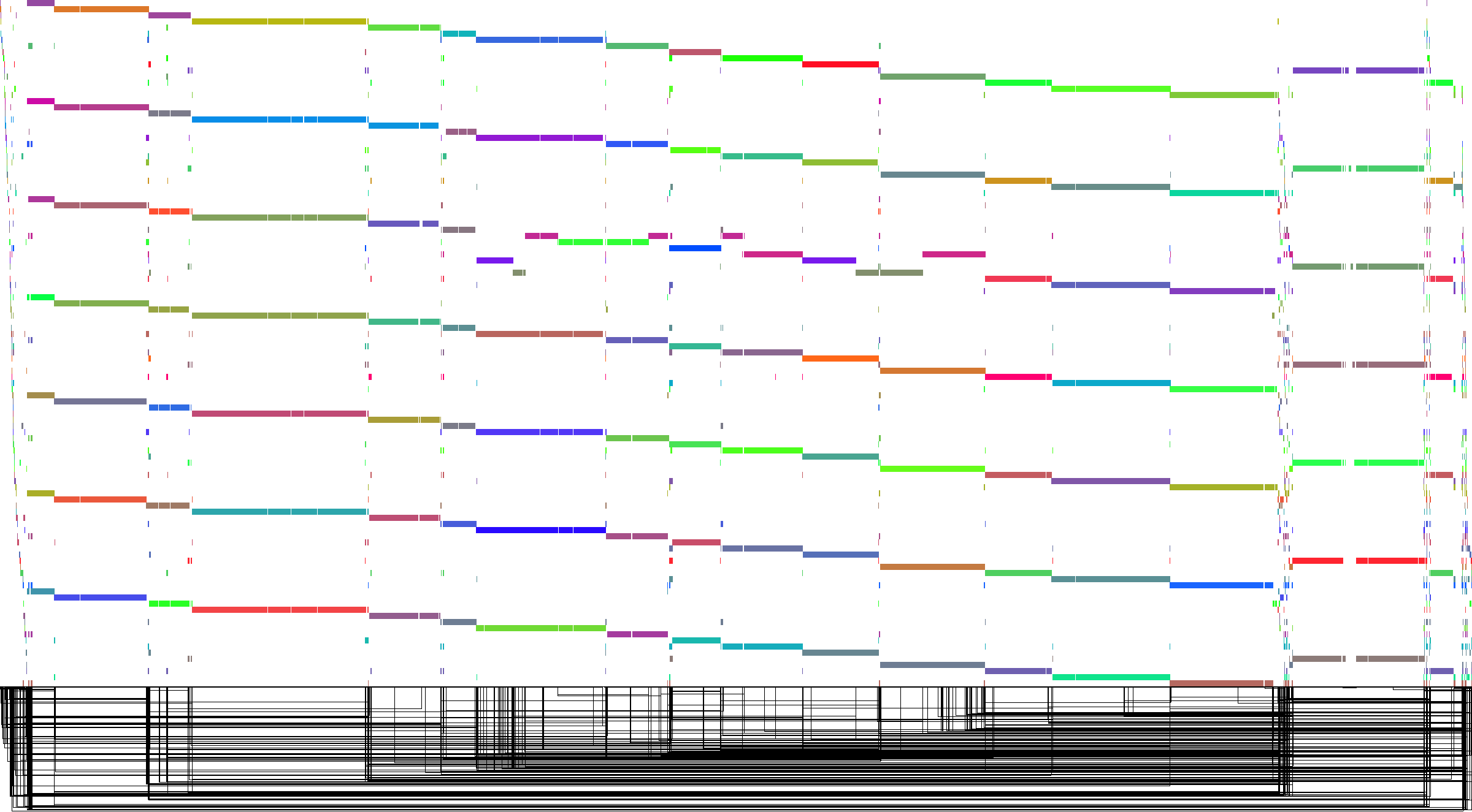
However, with odgi viz, we can obtain an image of how the embedded chromosomes relate to each other and to the topology of the graph.
This linear time rendering method displays the graph topology at the bottom of the image, using rectangular motifs to show where edges (hung below) link two positions in the sorted sequence space of the graph (the black line dividing the top and bottom of the image).
Paths are displayed above this topology, with one path at each position on the y axis.
The layout is nonlinear, and only shows what positions in the graph are touched by a given path.
But, because genome graphs are built from linear sequences, they have a manifold linear property and we can often apply a linear intuition to interpreting them.
In the following figure, genomes are ordered from top to bottom: S288c, DBVPG6765, UWOPS034614, Y12, YPS128, SK1, DBVPG6044. The chromosome order partly results from the initial sequential assignment of node ids by seqwish. We immediately see that a chromosome in UWOPS034614 (a highly diverged strain) has been rearranged into other chromosomes. Also notable are the frequent structural variations and CNVs that appear to be embedded in the ends of chromosomes. This confirms another finding from the paper describing these assemblies, whose authors observed that subtelomeric regions were hotspots of structural variation.
If you’re curious how this works, I’ve documented steps to do this for the whole collection. In the coming weeks, I’ll be reporting more on these methods and their applications to collections of human genome assemblies.
Working with other pangenomic methods
I was partly motivated to write this post by Heng Li’s release of a similar toolchain for the construction of pangenomic reference graphs. This approach is the first practical implementation of ideas about coordinate systems and reference graphs that arose during the GA4GH graph genome conversations. Heng proposes that we need a new data model to encode stable coordinates in pangenomes. This model (implemented in rGFA) is akin to the “side graph” that was discussed in those days, and also to the hierarchical model used by Seven Bridges Genomics. It annotates GFA elements with information that indicates their origin in a coordinate hierachy that has been constructed progressively. In effect, rGFA will be able to support the full range of semantics that we maintain in GFA, but it simplifies the process of relating stable coordinate systems into the graph using these annotations. rGFA provides a formal specification for the exchange of path relative coordinates that we have long been caching in various indexes used by tools in the vg ecosystem, and that may be very important for users of pangenomic models.
Heng also puts forward a prototype progressive pangenome construction algorithm (minigraph) that builds the graph to contain only structurally novel sequences relative to an established reference or graph that is being extended. minigraph is beautiful manifestation of Heng’s commitment to simple, efficient, and conceptually clean bioinformatic methods. Its performance is particularly motivating (I measure it as 5-10x faster than the seqwish pipeline), and provided it is based on minimap2 chaining, I would expect the resulting graphs to be of high quality in terms of capturing the large scale relationships between sequences. I am very happy that there is now another method to build pangenomes that can scale to the problem sizes that I’m working at, and I expect to be working with the output of minigraph in my own workflows.
However, I want to point out that there is a stark difference between what minigraph produces and the pangenomic models I’ve laid out here. Users of this method should understand that this is not a general solution to recording collections of genomes in a pangenome, but a way of deriving a coordinate hierarchy that relates to novel sequences according to a given progressive alignment model. I fear that, if taken up as the primary pangenomic model, the minigraph approach in its current form will perpetuate a long cycle of reference bias that has dominated many aspects of genomics since the establishment of resequencing based methods.
Minigraph pangenomes are lossy relative to their input sequences. It will not be possible to build a minigraph that contains all of the sequence in a set of samples unless there are no small variants between these sequences. The sequence included in the graph will be order dependent. This exposes us to reference bias for all kinds of variation that are not sufficiently large or divergent to frustrate the progressive alignment algorithm. The exact configuration that will trigger this may be opaque to end users. In these graphs we will have trouble knowing when we should expect to find a variant on this or that side of a bubble, or knowing for certain that a given variant has not been seen before based on read alignment to the graph.
In minigraph based graphs, we don’t have any small variation. This simplifies things and allows us to use legacy algorithms (sequence to sequence chaining and mapping) in the graph, but our results show that this will come at a cost in terms of accuracy for alignment to variants excluded from the graph. This also means that working with small variation in the context of minigraph references will require generalizations of VCF, and will retain all of the complexity related to that format. The effect of this will be to shift the difficulty of genotyping from alignment (as in graph genomes) back to variant calling (as in linear genomes).
The coordinate model that Heng proposes will provide a stable hierarchy, but only if the graph was constructed in the same way, by the same algorithm, or if the graph is a strict extension of a previous graph. Changes to the base reference will make the graphs incompatible. Because of this inflexibility, I do not believe that we should embed the coordinate system we use in the structure of the graph. Rather the two should be independent, allowing diverse graph structures to be built and used as needed during research even as we maintain a common coordinate space. All that is needed to provide coordinates (in variation graph terms) is a set of paths that mostly cover the graph. And that suggests how these models can work together. With minigraph, we can build a base rGFA that provides a covering coordinate space for the graph. Then, embedding these coordinate spaces as paths in our graph, we can decorate, extend, or rebuild the graph as we please, with whatever variation and genomes are useful for our analysis. This is all easy, because we’re already reading and writing the same format (GFA), although this exchange may not always be bidirectional due to algorithm limitations.
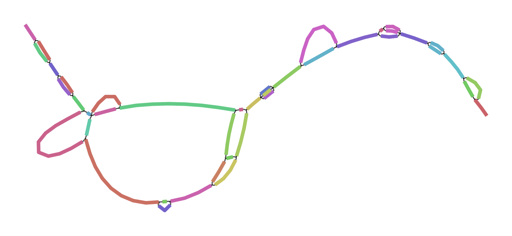
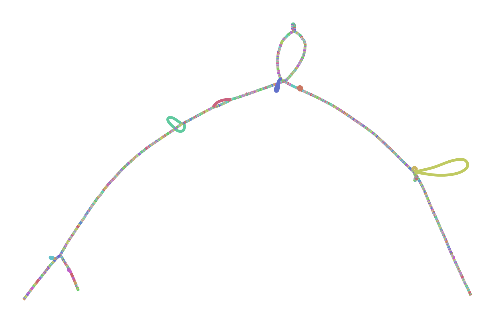
To make all this concrete, I leave you with two versions of the GRCh38 ALTs for DRB1-3123 in HLA. This gene is highly divergent in the human population, and I’ve long used it as a test during development and exploration with vg. The top graph was produced by minigraph, using a shorter (2kb) alignment threshold than default, while the bottom was produced by seqwish, with the same 2kb alignment filter. They are different in size (minigraph yields 20% more sequence in the graph) and complexity (seqwish is much more complex topologically) but suggest the same structure.
I look forward to working with Heng and the rest of the community to understand the best way to build and use these objects. I believe that this will require competitive but supportive and participant-oriented projects in which we not only build, but use pangenomes to drive genomic inference. Together, I am sure we will figure out how to bring these ideas to fruition and build scalable and helpful pangenomic methods. The important thing is that we learn to read and write the same data types. And, crucially, I hope that these data types are general enough to support all the things that researchers might need to do. There are exciting times ahead!
corrections
2019-07-10: I have updated this post to properly distinguish rGFA and minigraph and to resolve an error in the variation graph editing figure.